Pytorch part 1 - tensor and Pytorch tensor
This notebook introduces fundamental pieces of neural network such as tensors, Pytorch tensor operation, GPU, CUDA.


- Section 1: Introducing Pytorch, CUDA and GPU
- Section 2: Introducing Tensors
- Section 3: Pytorch Tensors
- Section 4: Pytorch Tensor Operation Types
- Random topics
- References
Section 1: Introducing Pytorch, CUDA and GPU
PyTorch is a deep learning framework and a scientific computing package.
The scientific computing aspect of PyTorch is primarily a result PyTorch’s tensor library and associated tensor operations. That means you can take advantage of Pytorch for many computing tasks, thanks to its supporting tensor operation, without touching deep learning modules.
Important to note that PyTorch tensors and their associated operations are very similar to numpy n-dimensional arrays. A tensor is actually an n-dimensional array.
Pytorch build its library around Object Oriented Programming(OOP) concept. With object oriented programming, we orient our program design and structure around objects (take a look at Random topics for more information). The tensor in Pytorch is presented by the object torch.Tensor which is created from numpy ndarray objects. Two objects share memory. This makes the transition between PyTorch and NumPy very cheap from a performance perspective.
With PyTorch tensors, GPU support is built-in. It’s very easy with PyTorch to move tensors to and from a GPU if we have one installed on our system. Tensors are super important for deep learning and neural networks because they are the data structure that we ultimately use for building and training our neural networks.
Talking a bit about history.
The initial release of PyTorch was in October of 2016, and before PyTorch was created, there was and still is, another framework called Torch which is also a machine learning framework but is based on the Lua programming language. The connection between PyTorch and this Lua version, called Torch, exists because many of the developers who maintain the Lua version are the individuals who created PyTorch. And they have been working for Facebook since then till now.
Below are the primary PyTorch modules we’ll be learning about and using as we build neural networks along the way.
| Package | Description |
|---|---|
| torch | The top-level PyTorch package and tensor library. |
| torch.nn | A subpackage that contains modules and extensible classes for building neural networks. |
| torch.autograd | A subpackage that supports all the differentiable Tensor operations in PyTorch. |
| torch.nn.functional | A functional interface that contains operations used for building neural net like loss, activation, layer operations... |
| torch.optim | A subpackage that contains standard optimization operations like SGD and Adam. |
| torch.utils | A subpackage that contains utility classes like data sets and data loaders that make data preprocessing easier. |
| torchvision | A package that provides access to popular datasets, models, and image transformations for computer vision. |
Why use PyTorch for deep learning?
- PyTorch’s design is modern, Pythonic. When we build neural networks with PyTorch, we are super close to programming neural networks from scratch. When we write PyTorch code, we are just writing and extending standard Python classes, and when we debug PyTorch code, we are using the standard Python debugger. It’s written mostly in Python, and only drops into C++ and CUDA code for operations that are performance bottlenecks.
- It is a thin framework, which makes it more likely that PyTorch will be capable of adapting to the rapidly evolving deep learning environment as things change quickly over time.
- Stays out of the way and this makes it so that we can focus on neural networks and less on the actual framework.
Why PyTorch is great for deep learning research
The reason for this research suitability is that Pytorch use dynamic computational graph, in contrast with tensorfow which uses static computational graph, in order to calculate derivatives.
Computational graphs are used to graph the function operations that occur on tensors inside neural networks. These graphs are then used to compute the derivatives needed to optimize the neural network. Dynamic computational graph means that the graph is generated on the fly as the operations are created. Static graphs that are fully determined before the actual operations occur.
It just so happens that many of the cutting edge research topics in deep learning are requiring or benefiting greatly from dynamic graphs.
Installing PyTorch
The recommended best option is to use the Anaconda Python package manager. With Anaconda, it's easy to get and manage Python, Jupyter Notebook, and other commonly used packages for scientific computing and data science, like PyTorch!
Let’s go over the steps:
- Download and install Anaconda (choose the latest Python version).
- Go to PyTorch's site and find the get started locally section.
- Specify the appropriate configuration options for your particular environment.
- Run the presented command in the terminal to install PyTorch
For the example:
conda install pytorch torchvision cudatoolkit=10.0 -c pytorch
Notice that we are installing both PyTorch and torchvision. Also, there is no need to install CUDA separately. The needed CUDA software comes installed with PyTorch if a CUDA version is selected in step (3). All we need to do is select a version of CUDA if we have a supported Nvidia GPU on our system.
!conda list torch
import torch
torch.__version__ # to verify pytorch version
torch.cuda.is_available() # to verify our GPU capabilities
Why deep learning uses GPUs
To understand CUDA, we need to have a working knowledge of graphics processing units (GPUs). A GPU is a processor that is good at handling specialized computations. This is in contrast to a central processing unit (CPU), which is a processor that is good at handling general computations. CPUs are the processors that power most of the typical computations on our electronic devices.
A GPU can be much faster at computing than a CPU. However, this is not always the case. The speed of a GPU relative to a CPU depends on the type of computation being performed. The type of computation most suitable for a GPU is a computation that can be done in parallel.
Parallel computing is a type of computation where by a particular computation is broken into independent smaller computations that can be carried out simultaneously. The resulting computations are then recombined, or synchronized, to form the result of the original larger computation. The number of tasks that a larger task can be broken into depends on the number of cores contained on a particular piece of hardware. Cores are the units that actually do the computation within a given processor, and CPUs typically have four, eight, or sixteen cores while GPUs have potentially thousands.
So why deep learning uses them - Neural networks are embarrassingly parallel.
Tasks that embarrassingly parallel are ones where it’s easy to see that the set of smaller tasks are independent with respect to each other. Many of the computations that we do with neural networks can be easily broken into smaller computations in such a way that the set of smaller computations do not depend on one another. One such example is a convolution.
GPU, CUDA and Nvidia
GPU computing
In the beginning, the main tasks that were accelerated using GPUs were computer graphics. That's why we have the name graphics processing unit. But in recent years, many more varieties parallel tasks have emerged. One such task as we have seen is deep learning.
Deep learning along with many other scientific computing tasks that use parallel programming techniques are leading to a new type of programming model called GPGPU or general purpose GPU computing.
GPU computing practically began with the introduction of CUDA by NVIDIA and Stream by AMD. These are APIs designed by the GPU vendors to be used together with the hardware that they provide.
Nvidia is a technology company that designs GPUs, and they have created CUDA as a software platform that pairs with their GPU hardware making it easier for developers to build software that accelerates computations using the parallel processing power of Nvidia GPUs.
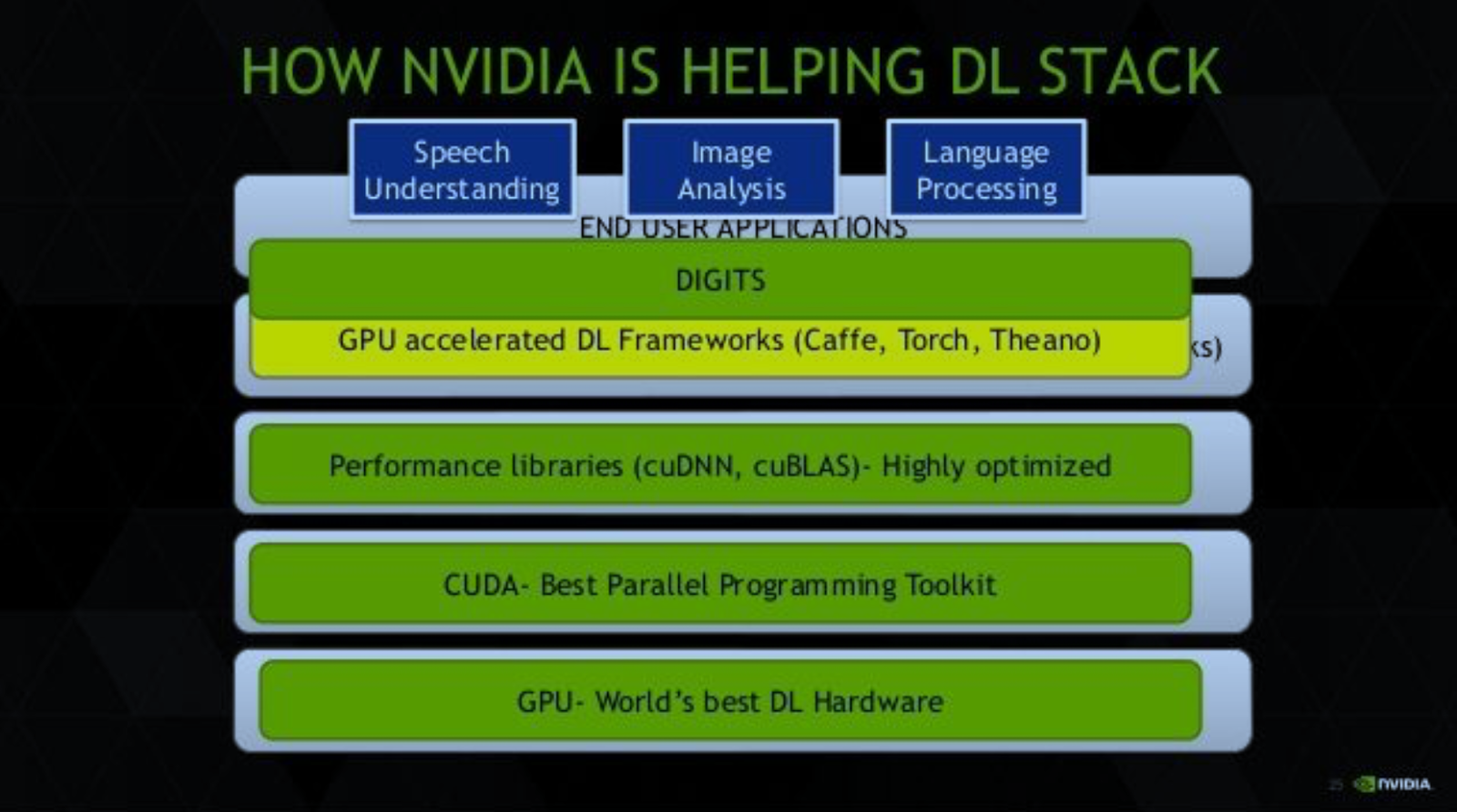
GPU computing stack concept
The stack comprises of:
- GPU as the hardware on the bottom
- CUDA as the software architecture on top of the GPU
- And finally libraries like cuDNN on top of CUDA.
Sitting on top of CUDA and cuDNN is PyTorch, which is the framework were we’ll be working that ultimately supports applications on top.
Developers use CUDA by downloading the CUDA toolkit which comes with specialized libraries like cuDNN - the CUDA Deep Neural Network library. With PyTorch, CUDA comes baked in from the start. There are no additional downloads required. All we need is to have a supported Nvidia GPU, and we can leverage CUDA using PyTorch. We don’t need to know how to use the CUDA API directly.
After all, PyTorch is written in all of these: Python, C++, CUDA
Suppose we have the following code:
t = torch.tensor([1,2,3])
The tensor object created in this way is on the CPU by default. As a result, any operations that we do using this tensor object will be carried out on the CPU. Now, to move the tensor onto the GPU, we just write:
t = t.cuda()
This ability makes PyTorch very flexible because computations can be selectively carried out either on the CPU or on the GPU.
Tensors - Data Structures of Deep Learning
A tensor is the primary data structure used by neural networks. The inputs, outputs, and transformations within neural networks are all represented using tensors, and as a result, neural network programming utilizes tensors heavily.
The below concepts, that we met in math or computer science, are all refered to tensor in deep learning.
| indexes required | math | computer science |
|---|---|---|
| 0 | scalar | number |
| 1 | vector | array |
| 2 | matrix | 2d-array |
The relationship within each of these pairs, for example vector and array, is that both elements require the same number of indexes to refer to a specific element within the data structure.
# an array or a vector requires 1 index to access its element
a = [1,2,3,4]
a[3]
# an matrix or 2d-array requires 2 index to access its element
a = [
    [1, 2, 3, 4],
    [5, 6, 7, 8]
]
a[0][2]
When more than two indexes are required to access a specific element, we stop giving specific names to the structures, and we begin using more general language.
- In mathematics, we stop using words like scalar, vector, and matrix, and we start using the word
tensorornd-tensor. The n tells us the number of indexes required to access a specific element within the structure. - In computer science, we stop using words like, number, array, 2d-array, and start using the word
multidimensional arrayornd-array. The n tells us the number of indexes required to access a specific element within the structure.
The reason we say a tensor is a generalization form is because we use the word tensor for all values of n like so:
- A scalar is a 0 dimensional tensor
- A vector is a 1 dimensional tensor
- A matrix is a 2 dimensional tensor
- A nd-array is an n dimensional tensor
The rank of a tensor refers to the number of dimensions present within the tensor. A rank-2 tensor means all of the following: a matrix, a 2d-array, a 2d-tensor.
An axis of a tensor is a specific dimension of a tensor.
Let's get an example how to access elements of an axis.
dd = [
[1,2,3],
[4,5,6],
[7,8,9]
]
Each element along the first axis, is an array:
dd[0], dd[1], dd[2]
Each element along the second axis, is a number:
dd[0][0], dd[1][0], dd[2][0]
The shape of a tensor gives us the length of each axis of the tensor.
reshaping.
t = torch.tensor([
    [1,2,3],
    [5,6,7]
], dtype=torch.float)
t.shape
Section 3: Pytorch Tensors
PyTorch tensors are the data structures we'll be using when programming neural networks in PyTorch.
The tensor in Pytorch is presented by the object torch.Tensor which is created from numpy ndarray objects. Two objects share memory. This makes the transition between PyTorch and NumPy very cheap from a performance perspective.
When programming neural networks, data preprocessing is often one of the first steps in the overall process, and one goal of data preprocessing is to transform the raw input data into tensor form.
t = torch.Tensor()
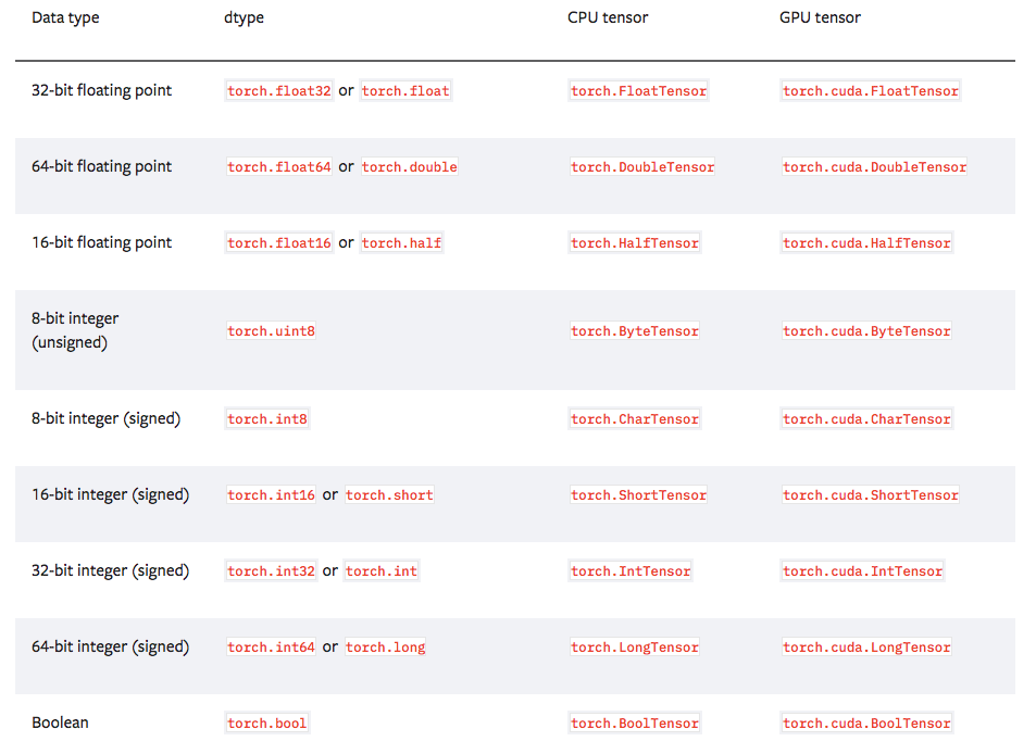
The dtype specifies the type of the data that is contained within the tensor.
t.dtype
Table below shows all the tensor types that Pytorch supports. Each type has a CPU and GPU version. Tensors contain uniform (of the same type) numerical data.
The device specifies the device (CPU or GPU) where the tensor's data is allocated. This determines where tensor computations for the given tensor will be performed.
t.device
PyTorch supports the use of multiple devices, and they are specified using an index like so:
device = torch.device('cuda:0')
device
If we have a device like above, we can create a tensor on the device by passing the device to the tensor’s constructor.
import torch
t = torch.tensor([1,2,3], dtype=torch.int, device=device)
The layout specifies how the tensor is stored in memory.
t.layout
To learn more about stride check here.
Create a new tensor using data
These are the primary ways of creating tensor objects (instances of the torch.Tensor class), with data (array-like) in PyTorch:
-
torch.Tensor(data) is the constructor of the
torch.Tensorclass -
torch.tensor(data): is the
factory functionthat constructstorch.Tensorobjects. - torch.as_tensor(data)
- torch.from_numpy(data)
Let’s look at each of these. They all accept some form of data and give us an instance of the torch.Tensor class. Sometimes when there are multiple ways to achieve the same result, things can get confusing, so let’s break this down.
import numpy as np
data = np.array([1,2,3])

o1 = torch.Tensor(data)
o2 = torch.tensor(data)
o3 = torch.as_tensor(data)
o4 = torch.from_numpy(data)

print(o1)
print(o2)
print(o3)
print(o4)
The table below compare 4 options and propose which one to use.
-
torch.tensoris best option to go daily ^^. It copy data which help us prevent hidden mistake caused by sharing data. In addition, it is better thantorch.Tensorthanks to better doc and more config options. -
torch.as_tensoris recommened in case we want to improve the performance and want to levarage data share memory characteristic of Pytorch. However, it is always better to start with copy data to make sure your program works first and go to performance improvement later. This option is better thantorch.from_numpybecause it accepts a wide variety of array-like objects including other Pytorch tensor.
| method | which one to use | dtype | data in memory |
|---|---|---|---|
| torch.Tensor(data) | infer from default dtype. | copy | |
| torch.tensor(data) | best option to go | inferred from input or explicitly set. | copy |
| torch.as_tensor(data) | use for improve performance | inferred from input or explicitly set. | share |
| torch.from_numpy(data) | inferred from input or explicitly set. | share |
Data in memory is shared means that the actual data in memory exists in a single place. As a result, any changes that occur in the underlying data will be reflected in both objects, the torch.Tensor and the numpy.ndarray.
Sharing data is more efficient and uses less memory than copying data because the data is not written to two locations in memory.
However, there are something to keep in mind about memory sharing:
- Since
numpy.ndarrayobjects are allocated on the CPU, theas_tensor()function must copy the data from the CPU to the GPU when a GPU is being used. - The memory sharing of
as_tensor()doesn’t work with built-in Python data structures likelist. - The
as_tensor()call requires developer knowledge of the sharing feature. This is necessary so we don’t inadvertently make an unwanted change in the underlying data without realizing the change impacts multiple objects. - The
as_tensor()performance improvement will be greater if there are a lot of back and forth operations betweennumpy.ndarrayobjects and tensor objects. However, if there is just a single load operation, there shouldn’t be much impact from a performance perspective.
Tips, In order to convert multiple arrays to tensor we can use map
import numpy as np
import torch

a = np.array([1,2,3])
b = np.array([3,4,5])
c = np.array([1])

a, b, c = map(torch.tensor, (a, b, c))
a, b, c
# create identity matrix
torch.eye(2)
# create a tensor of zeros with the shape of specified shape argument
torch.zeros([2,2])
# create a tensor of ones with the shape of specified shape argument
torch.ones([2,2])
# Returns a tensor filled with random numbers from a uniform distribution on the interval [0, 1)
# The shape of the tensor is defined by the variable argument size.
torch.rand([2,2])
# Returns a tensor filled with random numbers from a normal distribution with mean 0 and variance 1
# (also called the standard normal distribution).
torch.randn(2, 3)
This is a small subset of the available creation functions that don’t require data. Check with the PyTorch documentation for the full list.
Section 4: Pytorch Tensor Operation Types
We have the following high-level categories of tensor operations:
- Reshaping operation type: gave us the ability to position our elements along particular axes.
- Element-wise operation type: allow us to perform operations on elements between two tensors.
- Reduction operation type: allow us to perform operations on elements within a single tensor.
- Access operation type allow us to access to each numerical elements within a single tensor.
There are a lot of individual operations out there, so much so that it can sometimes be intimidating when you're just beginning, but grouping similar operations into categories based on their likeness can help make learning about tensor operations more manageable.
broadcasting
t1 = torch.tensor([
    [1,1],
    [1,1]
], dtype=torch.float32)

t2 = torch.tensor([2,4], dtype=torch.float32)

t1.shape, t2.shape
What will be the result of this element-wise addition operation, t1 + t2 ?
t1 + t2
Even though these two tenors have differing shapes, the element-wise operation is possible, and broadcasting is what makes the operation possible. The lower rank tensor t2 will be transformed via broadcasting to match the shape of the higher rank tensor t1, and the element-wise operation will be performed as usual.
we can check the broadcast transformation using the broadcast_to() numpy function.
import numpy as np
np.broadcast_to(t2.numpy(), t1.shape)
t1 + t2
After broadcasting, the addition operation between these two tensors is a regular element-wise operation between tensors of the same shape.
Using the reshape() function, we can specify the row x column shape that we are seeking. Notice that the product of the shape's components has to be equal to the number of elements in the original tensor.
Pytorch has another function called view() that does the same thing as reshape function.
import torch
t = torch.tensor([
    [1,1,1,1],
    [2,2,2,2],
    [3,3,3,3]
], dtype=torch.float32)
t.reshape([3,4])
Another common reshape type operation is squeeze, unsqueeze. Those operations change the shape of our tensors is by squeezing and unsqueezing them.
- Squeezing a tensor removes the dimensions or axes that have a length of one.
- Unsqueezing a tensor adds a dimension with a length of one.
t.reshape([1,12]).shape
t.reshape([1,12]).squeeze().shape
t.reshape([1,12]).unsqueeze(dim=0).shape
Another common reshape type operation is flattening.
A tensor flatten operation is a common operation inside convolutional neural networks. This is because convolutional layer outputs that are passed to fully connected layers must be flatted out before the fully connected layer will accept the input.
A flatten operation on a tensor reshapes the tensor to have a shape that is equal to the number of elements contained in the tensor. This is the same thing as a 1d-array of elements.
These are some ways to flatten a tensor.
t.reshape(1,-1)[0]
t.reshape(-1)
t.view(t.numel())
t.flatten()
In addition, it is possible to flatten only specific parts of a tensor.
t = torch.tensor([[
    [1,1,1,1],
    [2,2,2,2],
    [3,3,3,3]
]], dtype=torch.float32)
t.shape
t.flatten(start_dim=1).shape
Take a deeper look inside the flatten operation, it is actually a composition of reshape and squeeze operation.
def flatten_ex(t):
    t = t.reshape(1, -1)
    t = t.squeeze()
    return t
flatten_ex(t)
t1 = torch.tensor([[1,2],
                   [3,4]], dtype=torch.float32)
t2 = torch.tensor([[9,8],
                   [7,6]], dtype=torch.float32)
t1 + t2 # equivalent with t1.add(t2)
t1 + 2 # equivalent with t1.add(2)
t1 - 2 # equivalent with t1.sub(2)
t1 * 2 # equivalent with t1.mul(2)
t1 / 2 # equivalent with t1.div(2)
Comparison Operation is element-wise type operation
t.eq(0)
t.gt(0)
t.lt(0)
With element-wise operations that are functions, it’s fine to assume that the function is applied to each element of the tensor.
t.abs()
t.sqrt()
t.neg()
t.neg().abs()
A reduction operation on a tensor is an operation that reduces the number of elements contained within the tensor. Tensors give us the ability to manage our data. The tensor can be reduced to a single scalar value or reduced along an axis.
Let’s look at common tensor reduction operations:
import torch

t = torch.tensor([
    [0,1,0],
    [2,0,2],
    [0,3,0]
], dtype=torch.float32)
Reducing to a tensor with a single element
t.sum(), t.prod(), t.mean(), t.std()
Reducing tensors By Axes
t.sum(dim=0)
Argmax tensor reduction operation is very common in neural network.
This operation returns the index location of the maximum value inside a tensor.
In practice, we often use the argmax() function on a network’s output prediction tensor, to determine which category has the highest prediction value.
t.max(dim=1)
t.argmax(dim=1)
t.mean().item()
t.mean(dim=0).tolist()
t.mean(dim=0).numpy()
When we’re writing programs or building software, there are two key components, code and data. With object oriented programming, we orient our program design and structure around objects.
Objects are defined in code using classes. A class defines the object's specification or spec, which specifies what data and code each object of the class should have.
When we create an object of a class, we call the object an instance of the class, and all instances of a given class have two core components:
- Methods(code)
- Attributes(data)
In a given program, many objects, a.k.a instances of a given class have the same available attributes and the same available methods. The difference between objects of the same class is the values contained within the object for each attribute. Each object has its own attribute values. These values determine the internal state of the object. The code and data of each object is said to be encapsulated within the object.
Let’s build a simple class to demonstrate how classes encapsulate data and code:
class Sample: #class declaration
    def __init__(self, name): #class constructor (code)
        self.name = name #attribute (data)

    def set_name(self, name): #method declaration (code)
        self.name = name #method implementation (code)
Let's switch gears now and look at how object oriented programming fits in with PyTorch.
The primary component we'll need to build a neural network is a layer, and so, as we might expect, PyTorch's neural network library contains classes that aid us in constructing layers. As we know, deep neural networks are built using multiple layers. This is what makes the network deep. Each layer in a neural network has two primary components:
- A transformation (code)
- A collection of weights (data)
Like many things in life, this fact makes layers great candidates to be represented as objects using Object Oriented Programming - OOP.
References
Some good sources:
- pytorch zero to all
- deeplizard
- effective pytorch
- what is torch.nn really?
- recommend walk with pytorch
- official tutorial
- DL(with Pytorch)
- Pytorch project template
- nlp turorial with pytorch
- UDACITY course
- awesome pytorch list
- deep learning with pytorch
- others:
- https://medium.com/pytorch/get-started-with-pytorch-cloud-tpus-and-colab-a24757b8f7fc
- Grokking Algorithms: An illustrated guide for programmers and other curious people 1st Edition