Machine Learning with Graph - Preliminaries part 2
This notebook covers network properties and some random graph models. Primary source is from Standford CS224W course.


- Network Properties: How to Measure a Network
- Erdos-Renyi Random Graph Model
- The Small-World Model
- Kronecker Graph Model
- References
This is my personal notes for The Standford CS224W Course: Machine Learning with Graphs - Fall 2019 which I have been studying from its public resources for a couple of months. I will try to keep this blog series live update as my main source knowlege about graph. The course covers tremendous knowledge for understanding and effectively learning from large-scale network. In general, it is organized into 3 big sections:
-
preliminaries: provides basic background about networks/graphs. -
network methods: methods and algorithms which help us dealing with graph data structure. -
machine learning with networks: showing how we are applying machine learning into this field.
This notebook is part 2 of the preliminary section in which we will talk about network properties and some random graph models.
Here is the link to other parts: 1.
In this section, we will take a look on four key network properties which can be used to characterize a graph. These properties are extremely useful when we want to compare our model and real-world networks to see whether it fits.
- Degree Distribution: $P(k)$
- Path Length: $h$
- Clustering Coefficient: $C$
- Connected Components: $s$
The definitions will be presented for undirected graphs, but can be easily extended to directed graphs.
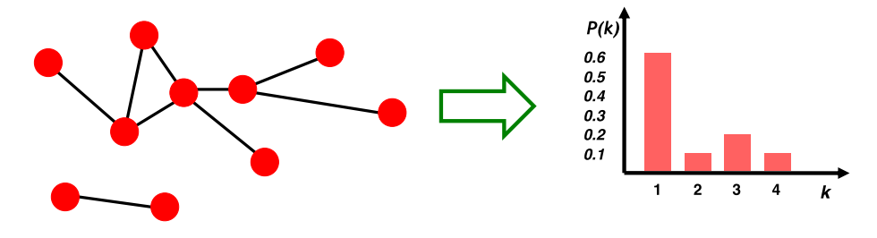
The degree distribution $P(k)$ measures the probability that a randomly chosen node has degree $k$.
The degree distribution of a graph $G$ can be summarized by a normalized histogram, where we normalize the histogram by the total number of nodes. We can compute the degree distribution of a graph by:
\begin{equation}
P(k)=\frac{N_k}{N}, N_{k}=\#nodes\_with\_degree\_k, N=\#nodes\_in\_graph
\end{equation}
A path is a sequence of nodes in which each node is linked to the next one: \begin{equation} P_{n}=\left\{i_{0}, i_{1}, i_{2}, \ldots, i_{n}\right\} \\ \end{equation} such that $\left\{\left(i_{0}, i_{1}\right),\left(i_{1}, i_{2}\right),\left(i_{2}, i_{3}\right), \ldots,\left(i_{n-1}, i_{n}\right)\right\} \in E$
In a directed graph, paths need to follow the direction of the arrows. Thus, distance is not symmetric for directed graphs. For a graph with weighted edges, the distance is the minimum number of edge weight needed to traverse to get from one node to another.
The Diameter of a graph is the maximum(shortest path) distance between any pair of nodes in a graph. The average path length for a connected graph or a strongly connected directed graph is the average shortest path between all connected nodes. We compute the average path length as: \begin{equation} \hat{h}=\frac{1}{2E_{\max}} \sum_{i, j \neq i} h_{i j} \end{equation} where:
$E_{max}$ is the max number of edges or node pairs; that is, $E_{max}=\left(\begin{array}{c}N \\ 2\end{array}\right)=\frac{N(N-1)}{2}$.
$h_{ij}$ is the distance from node $i$ to node $j$.
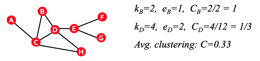
The clustering coefficient (for undirected graph) measures what proportion of node $i$'s neighbors are connected. For node $i$ with degree $k_i$, we compute the clustering coeffient as
\begin{equation}
C_i = \frac{2e_i}{k_i(k_i-1)}, C_{i} \in [0,1]
\end{equation}
where:
$e_i$ is the number of edges between the neighbors of node $i$.
$\frac{k_{i}(k_{i}-1)}{2}$ is the maximum number of edges between the $k_i$ neighbors
We can also compute the average clustering coefficient as \begin{equation} C = \frac{1}{N} \sum_{i}^{N} C_{i}. \end{equation}
The average clustering coefficient allows us to see if edges appear more densely in parts of the network. In social networks, the average clustering coefficient tends to be very high indicating that, as we expect, friends of friends tend to know each other.
The connectivity of a graph measures the size of the largest connected component. The largest connected component is the largest set where any two vertices can be joined by a path.
To find connected components:
- Start from a random node and perform breadth first search (BFS). If you are not familiar wit BFS, see here.
- Label the nodes that BFS visits
- If all the nodes are visited, the network is connected
- Otherwise find an unvisited node and repeat BFS
Now we will take a look at a real-world network, the protein-protein interation network, and see how much the four key properties are.
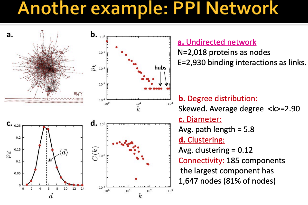
Some observations from this network are:
- The degree distribution is highly skewed, in a sense that majority of proteins have small degree and a few proteins have very high degree. On average, a node has around 3 neighbors.
- The diameter of this graph is around 6, it means within 6 steps you can reach any node in the (connected) graph. Does it surprise you? empirically, even with other networks with million of nodes, the diameter is also somewhere lower than 10. This characteristic relates to the concept of depth in graph neural network which we will see later.
- The average clustering is around 0.12, that means, on average, only around 10% of node's neightbors are connected one another.
- Lastly, the largest component has over 80% nodes of the network.
So are these values "expected"? Are they "surprising"?
So far we dont know, we need a model to see whether they are suprising or not. In the next part, we will go through some random graph models. Their power to model real-world networks is low but it helps us to have kind of baseline model to compare with other more powerful models. In addition, these random models are simple enough that we can calculate their properties by hand and see if a property can be easily obtained by random.
The Erdos-Renyi Random Graph Model is the simplest model of graphs. This simple model has proven networks properties and is a good baseline to compare real-world graph properties with.
This random graph model comes in two variants:
- $G_{np}$: undirected graph on $n$ nodes where each edge $(u,v)$ appears i.i.d with probability $p$.
- $G_{nm}$: undirected graph with $n$ nodes, and $m$ edges picked uniformly at random.
Note that both the $G_{np}$ and $G_{nm}$ graph are not uniquely determined, but rather the result of a random procedure. We can have many different realizations given the same $n$ and $p$
Let's take a look on the key properties of this random graph model.
The degree distribution of $G_{np}$ is binomial. Briefly remind, this distribution can be thought of as simply the probability of a SUCCESS or FAILURE outcome in an experiment that is repeated multiple times. It is a discrete analogue of a Gaussian and has a bell-shape. Binomial distribution has two variable: $n$ - number of times the experiment runs, $p$ - the probability of one specific outcome.

Recall that the clustering coefficient is computed as:
\begin{equation} C_{i}=2\frac{e_i}{k_{i}(k_{i}-1)} \end{equation}where $e_i$ is the number of edges between $i$'s neighbors. Edges in $G_{np}$ appear i.i.d with probability $p$, so the expected $e_i$ for $G_{np}$ is:
\begin{equation} \mathbb{E}\left[e_{i}\right]=p \frac{k_{i}\left(k_{i}-1\right)}{2} \end{equation}Thus, the expected clustering coefficient is
\begin{equation} \mathbb{E}\left[C_{i}\right]=\frac{p \cdot k_{i}\left(k_{i}-1\right)}{k_{i}\left(k_{i}-1\right)}=p=\frac{\bar{k}}{n-1} \approx \frac{\bar{k}}{n} \end{equation}where $\bar{k}$ is the average degree. From this, we can see that the clustering coefficient of $G_{np}$ is very small because $\bar{k}$ is really small compare to number of nodes $n$. If we generate bigger and bigger graphs with fixed average degree $\bar{k}$, then $C$ decreases with graph size $n$. \begin{equation} \mathbb{E}\left[C_{i}\right] \rightarrow 0, n \rightarrow \infty \end{equation}
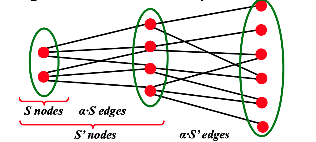
To discuss the path length of $G_{np}$, we first introduce the concept of expansion.
Graph $G(V, E)$ has expansion $\alpha$: if $\forall S \subset V$, the number of edges leaving $S \geq \alpha \cdot \min (|S|,|V \backslash S|)$ (for any subset of nodes, the number of edges leaving is greater than $\alpha$ * the length of subset). Expansion answers the question "if we pick a random set of nodes, how many edges are going to leave the set?". Expansion is a measure of robustness: to disconnect $l$ nodes, one must cut $\geq \alpha \cdot \ell $ edges.
Equivalently, we can say a graph $G(V, E)$ has an expansion $\alpha$ such that:
\begin{equation}
\alpha=\min _{S \subset V} \frac{\# \text { edges leaving } S}{\min (|S|,|V \backslash S|)}
\end{equation}
An important fact about expansion is that in a graph with $n$ nodes with expansion $\alpha$, for all pairs of nodes, there is a pair of path length $O((\log n) / \alpha)$ connecting them. Intuition, we can think of it like if we start with a subset of node and for each step the number of nodes visited increase with a factor of $\alpha$. Thus, it will take $\log n$ of steps to visit all nodes.
For the case of random graph $G_{np}$ and $\log n > np > c$, $c$ is a constant and $np$ is the average degree.
\begin{equation}
diam(G_{np}) = O(\frac{\log n}{\log (np)})
\end{equation}
Thus, we can see that random graphs have good expansion so it takes as logarithmic number of steps for BFS to visit all nodes.
Key thing to note, the path length of $G_{np}$ is $O(\log n)$. From this result, we can see that $G_{np}$ can grow very large, but nodes will still remain a few hops apart.
The graphic below shows the evolution of a $G_{np}$ random graph as $p$ change. We can see that there is an emergency of a giant component when average degree higher than 1.
- if $k=1-\epsilon$, then all components are of size $\Omega(\log n)$.
- if $k=1+\epsilon$, there exists 1 component of size $\Omega(n)$, and all other componnents have size $\Omega(\log n)$. In other words, if $\bar{k}>1$, we expect a single large component. In addition, in this case, each node has at least one edge in expectation.
So as average degree $k<1$, fraction of nodes in largest component does not change much but it will start to increase exponentially as $k>1$.

In order to see if our random model fits well with a real network, let's take a look on MSN Messenger network in 1 month of activify which has 180 million users and 1.3 billion edges.
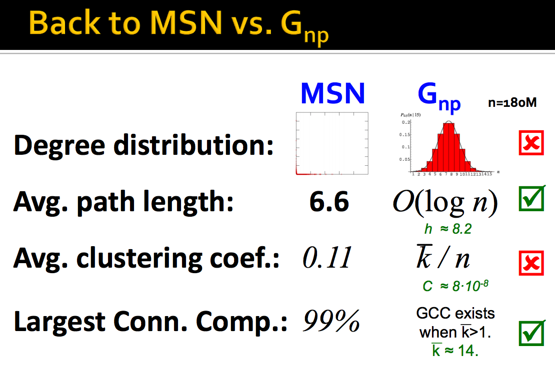
As we can see, giant connected component and average path length might fit between them but clustering coefficient and degree distribution do not. The problem with the random network model are:
- Degree distribution differs from that of real networks
- Giant component in most real networks does NOT emerge through a phase transition
- No local structure - clustering coefficient is too low. Thus, we can conclude that real networks obviously are not random.
Although the random network $G_{np}$ is WRONG to model real network but it is still useful because:
- It is the reference model for the rest of the class
- It will help us calculate many quantities, that can then be compared to the real data
- It will help us understand to what degree a particular property is the result of some random process.
This model is the improvement of random model in which it tackles the problem of constructing graph with low average path length and high clustering.
The Small-World model was first introduced in 1998 by Ducan J.Watts and Steven Strogatz. To create such model, we employ the following steps:
- Start with a low-dimensional regular lattice(ring) by connecting each node to $k$ neighbors on its right and $k$ neightbors on its left, with $k \geq 2$. So we have a lattice with high clustering coefficient.
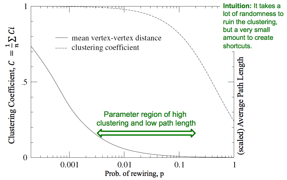
- Rewire each edge with probability $p$ by moving its endpoint to a randomly chosen node. This step will add/remove edges to create shortcuts to join remote parts of the lattice. So we are introducing randomness (shortcut) into the lattice. The rewiring allows us to "interpolate" between a regular lattice and a random graph.
Note: Clustering implies edge "locality". Randomness enables "shortcuts"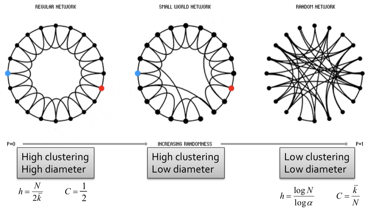
Then, we make the following observations:
- At $p=0$ where no rewiring has occured, this remains a grid network with high clustering, high diameter.
- For $0<p<1$ some edges have been rewired, but most of the structure remains. This implies both locality and shortcuts. This allows for both high clustering and low diameter.
- At $p=1$ where all edges have been randomly rewired, this is a Erdos-Renyi (ER) random graph with low clustering, low diameter.
Note: Small world model are parameterized by the probability of rewiring $p \in[0,1]$
From a social network perspective, the phenomenon of introducing shortcuts while keeping strong structure is intuitive. While most our friends are local, but we also have a few long distance friendships in different countries which is enough to collapse the diamter of the human social network, explaining the popular notion of Six Degrees of Separation".
In summary, the small world model:
- provides insight on the interplay between clustering and the small-world.
- captures the structure of many realistic networks.
- accounts for the high clustering of real networks.
- but it does not lead to the correct degree distribution of real-world network.
Models of graph generation have been studied extensively. Such models allow us to generate graphs for simulations and hypothesis testing when collecting the real graph is difficult, and also forces us to examine the network properties that generative models should obey to be considered realistic.
In formulating graph generation models, there are two important considerations:
- The ability to generate realistic networks.
- The mathematical tractability of the models, which allows for the rigorous analysis of network properties.
The Kronecker Graph Model is a recursive graph generation model that combines both mathematical tractability and realistic static and temporal network properties. The intuition underlying the Kronecker Graph Model is self-similarity, where the whole has the same shape as one or more of its parts.
The Kronecker product $\otimes$, a non-standard matrix operation, is a way of generating self-similar matrics. For two arbitarily sized matrices $\mathbf{A} \in \mathbb{R}^{n \times m}$ and $\mathbf{B} \in \mathbb{R}^{k \times l}, \mathbf{A} \otimes \mathbf{B} \in \mathbb{R}^{n k \times m l}$, their Kronecker product is: \begin{equation} \mathbf{C}={\mathbf{A}} \otimes \mathbf{B} \doteq\left(\begin{array}{cccc} a_{1,1} \mathbf{B} & a_{1,2} \mathbf{B} & \dots & a_{1, m} \mathbf{B} \\ a_{2,1} \mathbf{B} & a_{2,2} \mathbf{B} & \dots & a_{2, m} \mathbf{B} \\ \vdots & \vdots & \ddots & \vdots \\ a_{n, 1} \mathbf{B} & a_{n, 2} \mathbf{B} & \dots & a_{n, m} \mathbf{B} \end{array}\right) \end{equation}
For example, we have that $$\begin{bmatrix} 1&2\\3&4 \end{bmatrix} \otimes \begin{bmatrix} 0&5\\6&7 \end{bmatrix} = \begin{bmatrix} 1 \begin{bmatrix} 0&5\\6&7 \end{bmatrix} &2 \begin{bmatrix} 0&5\\6&7 \end{bmatrix} \\3 \begin{bmatrix} 0&5\\6&7 \end{bmatrix} &4 \begin{bmatrix} 0&5\\6&7 \end{bmatrix} \end{bmatrix} = \begin{bmatrix} 1 \times 0 & 1 \times 5 & 2 \times 0 & 2 \times 5\\ 1 \times 6 & 1 \times 7 & 2 \times 6 & 2 \times 7\\ 3 \times 0 & 3 \times 5 & 4 \times 0 & 4 \times 5\\ 3 \times 6 & 3 \times 7 & 4 \times 6 & 4 \times 7 \end{bmatrix} = \begin{bmatrix} 0 & 5 & 0 & 10\\ 6 & 7 & 12 & 14\\ 0 & 15 & 0 & 20\\ 18 & 21 & 24 & 28 \end{bmatrix}$$
To use the Kronecker product in graph generation, we define the Kronecker product of two graphs as the Kronecker product of the adjacency matrices of the two graphs.
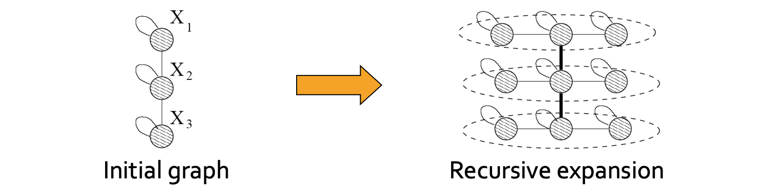
Kronecker graph is obtained by growing sequence of graphs by iterating the Kronecker product over the initiator matrix $K_1$ (an adjacency matrix of a graph):
$$K_1^{[m]}=K_m = \underbrace{K_1 \otimes K_1 \otimes \dots K_1}_{\text{m times}}= K_{m-1} \otimes K_1$$
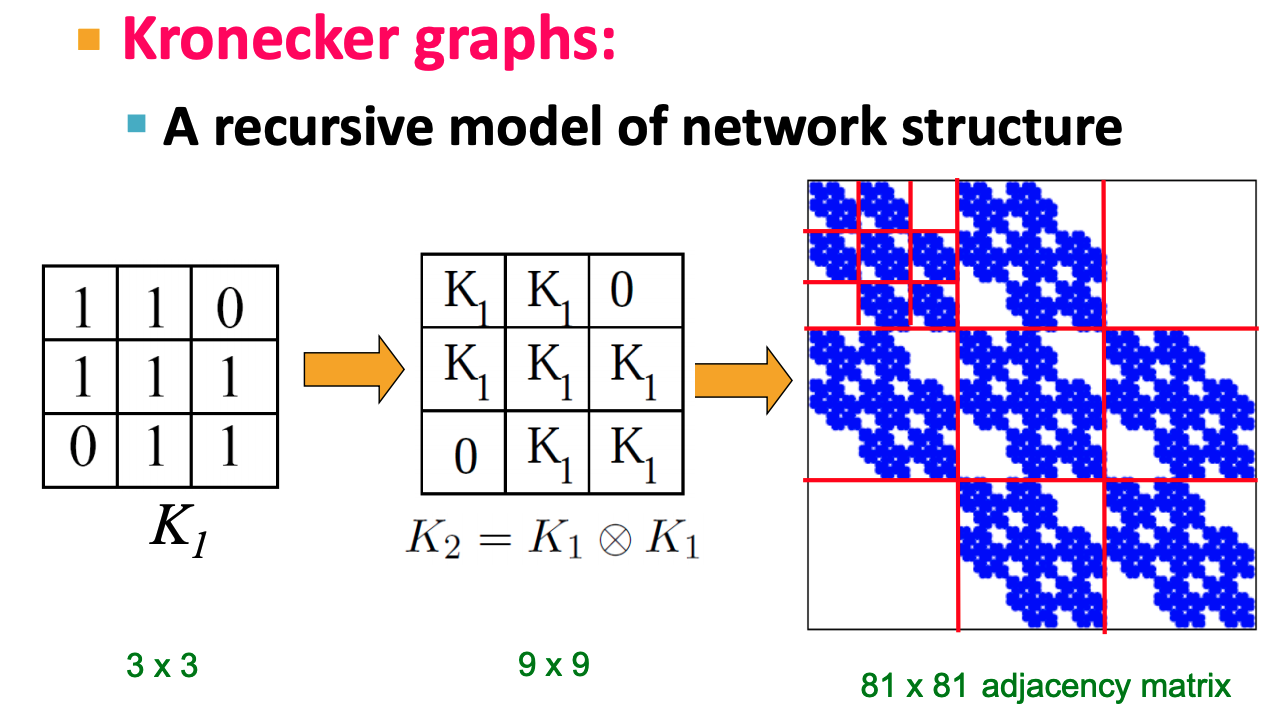
Intuitively, the Kronecker power construction can be imagined as recursive growth of the communities within the graph, with nodes in the community recursively getting expanded into miniature copies of the community.
One can easily use multiple initiator matrices $(K_{1}^{\prime}, K_{1}^{\prime \prime}, K_{1}^{\prime \prime \prime})$ (even of different sizes), which iteratively affects the structure of the larger graph.
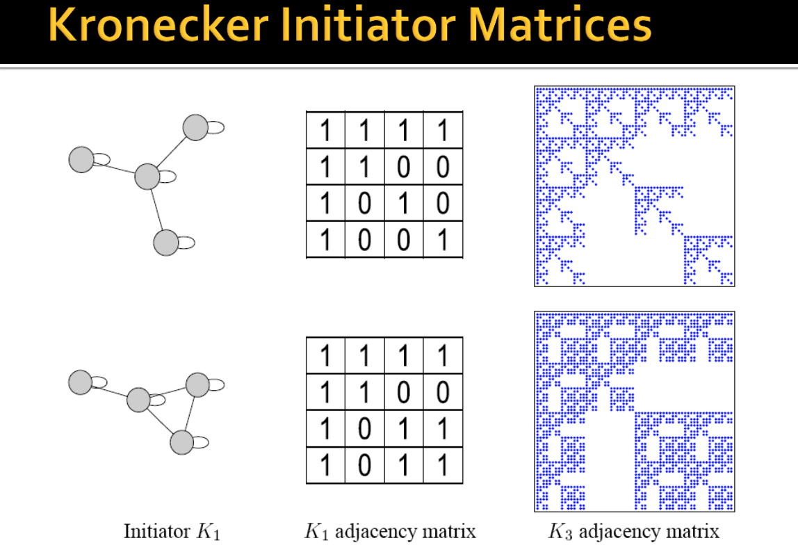
Up to now, we have only considered $K_1$ initiator matrices with binary values $\{0,1\}$. However, such graphs generated from such initiator matrices have "staircase" effects in the degree distributions and individual values occur very frequently because of the discrete nature of $K_1$.
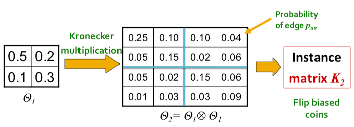
To negate this effect, stochasticity is introduced by relaxing the assumption that the entries in the initiator matrix can only take binary values. Instead entries in $\Theta_1$ can take values on the interval $[0, 1]$, and each represents the probability of that particular edge appearing. Then the matrix (and all the generated larger matrix products) represents the probability distribution over all possible graphs from that matrix.
More concretely, for probability matrix $\Theta_1$, we compute the $k^{th}$ Kronecker power $\Theta_k$ as the large stochastic adjacency matrix. Each entry $p_{uv}$ in $\Theta_k$ then represents the probability of edge $(u, v)$ appearing.
Notes:the probabilities do not have to sum up to 1 as each the probability of each edge appearing is independent from other edges.
To obtain an instance of a graph, we then sample from the distribution by sampling each edge with probability given by the corresponding entry in the stochastic adjacency matrix. The sampling can be thought of as the outcomes of flipping biased coins where the bias is parameterized from each entry in the matrix.
However, this means that the time to naively generate an instance is quadratic in the size of the graph, $O(N^2)$! too slow.
Is there a faster way?
A fast heuristic procedure that takes time linear in the number of edges to generate a graph exists.
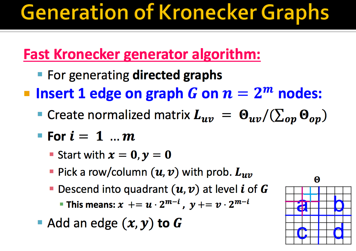
The general idea can be described as follows: for each edge, we recursively choose sub-regions of the large stochastic matrix with probability proportional to $p_{uv} \in \Theta_{1}$ until we descend to a single cell of the large stochastic matrix. We replace the edge there. For a Kronecker graph of $k^{th}$ power, $\Theta_k$, the descent will take $k$ steps.
For example, we consider the case where $\Theta_1$ is a $2 x 2$ matrix, such that
\begin{equation}
\Theta=\left[\begin{array}{ll}
a & b \\
c & d
\end{array}\right]
\end{equation}
For graph $G$ with $n = 2^k$ nodes, we need to define how many edges we want to generate (we can reference of the ratio between number of nodes and number of edges). Then, the algorithm to generate each edge is shown below:
In practice, the stochastic Kronecker graph model is able to generate graphs that match the properties of real world networks well. To read more about the Kronecker Graph models, refer to J Leskovec et al., Kronecker Graphs: An Approach to Modeling Networks (2010).
References
- main source: Standford CS224W Machine Learning with Graphs
- other sources
- Graph on structured documents blog post
- Graph theory blog post
- Graph embedding blog post
- Graph convolution blog post
- Geometric deep learning blog post
- review papers about graphs: 1, 2
- Pytorch Geometric:1, 2