Pytorch part 2 - neural net from scratch
This notebook will create and train a very simple model from scratch and then gradually refactor it using built-in pytorch modules.


- Section 1: data and data processing
- Section 2: create and train model (from scratch)
- Section 3: refactor model using Pytorch built-in modules
- Section 4: random topics
- Reference
In part 1 of this serie, we have gone through the basic elements of neural network. In this part we will start writing a program.
Computer programs in general consist of two primary components, code and data. With traditional programming, the programmer’s job is to explicitly write the software or code to perform computations. But with deep learning and neural networks, this job explicitly belongs to the optimization algorithm. It will compile our data into code which is actually neural net's weights. The programmer’s job is to oversee and guide the learning process though training. We can think of this as an indirect way of writing software or code.
In reality, creating and trainning model is just one of the stages in a fullscale machine learning project. There are 4 fundamental stages that a machine learning project need to have:
- Project planning and project setup: gather team, define requirements, goals and allocate resources.
- Data collection and labelling: define which data to collect and label them.
- Training and debugging: start implementing, debugging and improving model. This notebook will focus on this stage where we will create and train a simple model using Pytorch framework.
-
Deploying and testing write tests to prevent regresison, roll out in production.
Important: it is worth to note that machine learning project does not fit well with either waterfall or agile workflow. It is somewhere in between them and the world is in progress to figure out a new workflow for it. However, it can be sure that this type of project needs to be highly iteractive and flexible. We will try to cover this topic more detail in later parts of this serie.
So now we will go to the main topic today.
There are 3 steps that we need to iteractively tackle during the training and debugging stage:
- data and data processing: data augmentation, data transformation, data cleaning, etc
- create and train model guide the optimization algorithm toward the right direction.
- debug and improve: analyse model's results to see where might need to improve.
Debugging machine learning is always a hot topic and hard to digest, we will cover it in a separate notebook. Today we will talk about data and model, but not too fast. In order to fully understand exactly what and how things are doing, we will create and train a very basic neural network from scratch which initially only use the most basic Pytorch tensor functionality and gradually refactor it using Pytorch built-in modules.
Remind the most fundamental Pytorch modules which we will repeatly work with along the way.
| Package | Description |
|---|---|
| torch | The top-level PyTorch package and tensor library. |
| torch.nn | A subpackage that contains modules and extensible classes for building neural networks. |
| torch.autograd | A subpackage that supports all the differentiable Tensor operations in PyTorch. |
| torch.nn.functional | A functional interface that contains operations used for building neural net like loss, activation, layer operations... |
| torch.optim | A subpackage that contains standard optimization operations like SGD and Adam. |
| torch.utils | A subpackage that contains utility classes like data sets and data loaders that make data preprocessing easier. |
| torchvision | A package that provides access to popular datasets, models, and image transformations for computer vision. |
Data is the primary ingredient of deep learning. Before feeding data into our network, we need to consider many aspects such as:
- Who created the dataset?
- How was the dataset created?
- What transformations were used?
- What intent does the dataset have?
- Possible unintentional consequences?
- Is the dataset biased?
- Are there ethical issues with the dataset?
In this tutorial, we will use the well-prepared Fashion-MNIST dataset which was created by research lab of Zalando - a German based multi-national fashion commerce company. The dataset was designed to mirror the original MNIST dataset as closely as possible while introducing higher difficulty in training due to simply having more complex data than hand written images. The abstract from its paper:
We present Fashion-MNIST, a new dataset comprising of 28 × 28 grayscale images of 70, 000 fashion products from 10 categories, with 7, 000 images per category. The training set has 60, 000 images and the test set has 10, 000 images. Fashion-MNIST is intended to serve as a direct dropin replacement for the original MNIST dataset for benchmarking machine learning algorithms, as it shares the same image size, data format and the structure of training and testing splits. The dataset is freely available at https://github.com/zalandoresearch/fashion-mnist.
The Fashion-MNIST was built, unlike the hand-drawn MNIST dataset, from actual images on Zalando’s website. However, they have been transformed to more closely correspond to the MNIST specifications. This is the general conversion process that each image from the site went through:
- Converted to PNG
- Trimmed
- Resized
- Sharpened
- Extended
- Negated
- Gray-scaled
The dataset has the following ten classes of fashion items:
idx2clas = {0 : "T-shirt/top",
            1 : "Trouser",
            2 : "Pullover",
            3 : "Dress",
            4 : "Coat",
            5 : "Sandal",
            6 : "Shirt",
            7 : "Sneaker",
            8 : "Bag",
            9 : "Ankle boot"}
A sample of the items look like this:
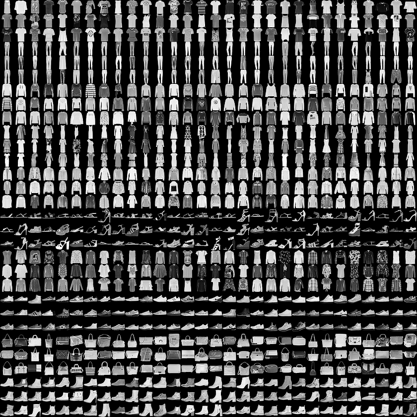
That's enough background information about the dataset. Now we will prepare data for our network.
The general idea of this step is to transform our dataset into tensor format so we can take advantages of GPU's parallel computing for later steps such as data augmentation, training model, etc.
We'll follow the ETL process to prepare data:
- Extract: Get the Fashion-MNIST image data from the source.
- Transform: Put our data into tensor form.
- Load: Put our data into an object to make it easily accessible.
The Fashion-MNIST source code can be accessed here. We will use pathlib for dealing with paths and will download 4 parts - training set images, training set labels, test set images and test set labels - using requests library. Since this dataset has been stored using pickle, a python-specific format for serializing data, we need to unzip and deserialize it in order to read the content.
# a. extract data from source

from pathlib import Path
import requests

PATH_ROOT = Path("data/fashion_mnist")
PATH_ROOT.mkdir(parents=True, exist_ok=True)

URLs = [
"http://fashion-mnist.s3-website.eu-central-1.amazonaws.com/train-images-idx3-ubyte.gz",
"http://fashion-mnist.s3-website.eu-central-1.amazonaws.com/train-labels-idx1-ubyte.gz",
"http://fashion-mnist.s3-website.eu-central-1.amazonaws.com/t10k-images-idx3-ubyte.gz",
"http://fashion-mnist.s3-website.eu-central-1.amazonaws.com/t10k-labels-idx1-ubyte.gz"
]

def download_data(path_root, url):
    filename = Path(url).name
    if not (path_root / filename).exists():
        content = requests.get(url).content
        (path_root / filename).open("wb").write(content)

for url in URLs: download_data(PATH_ROOT, url)
def load_data(path, kind='train'):
    import os
    import gzip
    import numpy as np

    """Load MNIST data from `path`"""
    labels_path = os.path.join(path,
                               '%s-labels-idx1-ubyte.gz'
                               % kind)
    images_path = os.path.join(path,
                               '%s-images-idx3-ubyte.gz'
                               % kind)

    with gzip.open(labels_path, 'rb') as lbpath:
        labels = np.frombuffer(lbpath.read(), dtype=np.uint8,
                               offset=8)

    with gzip.open(images_path, 'rb') as imgpath:
        images = np.frombuffer(imgpath.read(), dtype=np.uint8,
                               offset=16).reshape(len(labels), 784)

    return images, labels

x_train, y_train = load_data(PATH_ROOT, kind='train')
x_valid, y_valid = load_data(PATH_ROOT, kind='t10k')
valid and test interchanged but in reality they are different.
This dataset is in numpy array format. Each image is 28*28 and is being stored as a flattened row of length 784.
Let's reshape and take a look at one.
x_train.shape, y_train.shape
y_train.max(), y_train.min()
x_valid.shape, y_valid.shape
y_valid.max(), y_valid.min()
from matplotlib import pyplot as plt
import numpy as np

plt.imshow(x_train[0].reshape(28,28), cmap="gray")
idx2clas[y_train[0].item()]

So we have finished the extract data step and now we will to to transform step. In the context of image, there are 2 basic transform steps are convert to tensor and normalization. Normalization is a standard step in image processing which helps faster convergence.
import torch

# transform 1. convert to tensor
x_train, x_valid = map(lambda p: torch.tensor(p, dtype=torch.float32), (x_train, x_valid))
y_train, y_valid = map(lambda p: torch.tensor(p, dtype=torch.int64), (y_train, y_valid))
# transform 2. normalize images
mean = x_train.mean()
std = x_train.std()
print(f"mean: {mean}, std: {std}")
x_train, x_valid = map(lambda p: (p - mean)/std, (x_train, x_valid))
x_train.mean(), x_train.std()
x_valid.mean(), x_valid.std()
load data into an object to make it easily accessible. This task normally is handled by Pytorch DataLoader object but since we are building everything from scratch, let's use the traditional for loop to access batches of data.
# c. load batches of data
batch_size = 64
nr_iters = len(x_train) // batch_size

for i in range((nr_iters + 1)):
    start_index = i * batch_size
    end_index = start_index + batch_size
    xs = x_train[start_index:end_index]
    ys = y_train[start_index:end_index]
    print(xs.shape)
    print(ys.shape)
Section 2: create and train model (from scratch)
For our 10-class classification problem, we will create a simple network which contains only a linear layer and a non-linear layer - softmax.
In general, a layer contains 2 parts:
-
data: represents the state of that layer. In particular, they are weight and bias - learnable parameters which are updated/learned during training process. -
transformation: the operation which transform layer's input to output using learnable parameters.
Linear layers's data is weight matrix tensor and bias tensor while its transformation is the matrix multiplication. Weight matrix defines the linear function that maps a 1-dimentional tensor with 784 elements to a 1-dimensional tensor with 10 elements.
Weight matrix tensor, Input tensor, Bias tensor and Output tensor, respectively. Mathematical notation of a linear transformation is: $y=Ax+b$
The weight matrix tensor will be initialized following the recommendation from Xavier initialisation paper. This paper tackled the problem with randomly initialized weight drawn from Gaussian distribution which caused hard convergence for deep network.
requires_grad_ after initialization, since we don’t want that step included in the gradident. The trailing _ in Pytorch signifies that the operation is performed in-place.
import math

weights = torch.randn(784,10) / math.sqrt(784)
weights.requires_grad_()
bias    = torch.zeros(10, requires_grad=True)
Thanks to Pytorch's ability to calculate gradients automatically, we can use any standard Python function (or callable object) as a model.
The log_softmax function is implemented using log-sum-exp trick for numerically stable. We will not go to detail this trick but you can go here or here for details explanation. The formular for this trick is:
$$ log\_softmax(x) = x - logsumexp(x) $$
def log_softmax(x): return x - x.exp().sum(-1).log().unsqueeze(-1)
def simplenet(x): return log_softmax(x @ weights + bias)
@ stand for dot product operation.
bs = 16
xs, ys = x_train[:bs], y_train[:bs]
preds = simplenet(xs)
preds.shape
preds
What we have done is one forward pass, we load a batch of image add feed it through the network. The result will not be better than a random prediction at this stage because we start with random weights.
It can be seen in the preds tensor that it contains not only the tensor values but also a gradient function. As mentioned in part 1, pytorch use dynamic computational graph to track function operations that occur on tensors. These graph are then used to compute the derivatives.
preds.grad_fn
Now we need to define the loss function which is the model's objective. Our weights and bias will be updated in the direction which make this loss decreased. One of the most common loss function is negative log-likelihood.
def nll(input, target):
    return -input[range(input.shape[0]), target.tolist()].mean()

loss_function = nll

loss_function(preds, ys)
Next, We will define a metric. During the training, reducing the loss is what our model tries to do but it is hard for us, as human, can intuitively understand how good the weights set are along the way. So we need a human-interpretable value which help us understand the training progress and it is the metric.
def accuracy(input, target):
    return (torch.argmax(input, dim=1) == target).float().mean()

accuracy(preds, ys)
We are now ready to begin the training process. The training process is an iterative process which including following steps:
-
Get a batch from the training set.
- Since we have 60,000 samples in our training set, we will have 938 iterations with batch_size 64. Something to notice, batch_size will directly impact to the number of times the weights updated. In our case, the weights will be updated 938 times by the end of each loop. So far, there is no rule-of-thump for selecting the value of batch size so we still need to do trial and error to figure out the best value.
Important: to be simple, I am not shuffling the training set at this stage. In reality, the training set should be shuffled to prevent correlation between batches and overfitting. If we keep feeding the network batch-by-batch in an exact order many times, the network might remember this order and causes overfitting with it. On the other hand, the validation loss will be identical whether we shuffle the validation set or not. Since shuffling takes extra time, it makes no sense to shuffle the validation data.
- Since we have 60,000 samples in our training set, we will have 938 iterations with batch_size 64. Something to notice, batch_size will directly impact to the number of times the weights updated. In our case, the weights will be updated 938 times by the end of each loop. So far, there is no rule-of-thump for selecting the value of batch size so we still need to do trial and error to figure out the best value.
-
Pass batch to network.
-
Calculate the loss value.
-
Calculate the gradient of the loss function w.r.t the network's weights.
- Calculating the gradients is very easy using PyTorch. Since PyTorch has created a computation graph under the hood. As our batch tensor steps forward through our network, all the computations are recorded in the computational graph. And this graph is then used by PyTorch to calculate the gradients of the loss function with respect to the network's weights.
-
Update the weights.
- The gradients calculated from step 4 are used by the optimizer to update the respective weights.
- We have disabled PyTorch gradient tracking at this step because we don't want these actions to be recorded for our next calculation of the gradient. There are many ways to disable this functionality, please check
Random topicsat the end of notebook for more information. - After updating the weight, we need to zero out the gradients because the gradients will be calculated and added to the grad attributes of our network's parameters after calling
loss.backward()at the next iteration.
Note: Zero out the gradient after updating parameters is not always the case, there are some special cases where we want toaccumulate gradient. But you only have to deal with it at advance level. So take care^^.
-
Repeat steps 1-5 until one epoch is completed.
-
Calculate mean loss of validation set
Note: We can use a batch size for the validation set that is twice as large as that for the training set. This is because the validation set does not need backpropagation and thus takes less memory (it doesn’t need to store the gradients). We take advantage of this to use a larger batch size and compute the loss more quickly. - Repeat steps 1-6 for as many epochs required to reach the minimum loss.
We will use Stochastic Gradient Descent (SGD) optimizer to update our learnable parameters during training. lr tells the optimizer how far to step in the direction of minimizing loss function.
lr = 0.01
epochs = 5
batch_size = 64

nr_iters = len(x_train) // bs
for epoch in range(epochs):
    for i in range((nr_iters + 1)):
        # step 1. get batch of training set
        start_index = i * batch_size
        end_index = start_index + batch_size
        xs = x_train[start_index:end_index]
        ys = y_train[start_index:end_index]
        # step 2. pass batch to network
        preds = simplenet(xs)
        # step 3. calculate the loss
        loss = loss_function(preds, ys)
        # step 4. calculate the gradient of the loss w.r.t the network's parameters
        loss.backward()
        with torch.no_grad():
            # step 5. update the weights using SGD algorithm
            weights -= lr * weights.grad
            bias    -= lr * bias.grad
            weights.grad.zero_()
            bias.grad.zero_()
    # step 6. calculate mean of valid loss after each epoch to see the improvement
    batch_size_valid = batch_size * 2
    nr_iters_valid = len(x_valid) // batch_size_valid
    total_loss = 0
    total_acc  = 0
    with torch.no_grad():
        for i in range((nr_iters_valid + 1)):
            start_index = i * batch_size_valid
            end_index = start_index + batch_size_valid
            xs = x_valid[start_index:end_index]
            ys = y_valid[start_index:end_index]
            preds = simplenet(xs)
            loss = loss_function(preds, ys)
            total_loss += loss.item() * xs.shape[0]

            acc = accuracy(preds, ys)
            total_acc += acc.item() * xs.shape[0]
    print(f"epoch {epoch}, valid_loss {total_loss / len(x_valid)}, accuracy {total_acc / len(x_valid)}")
During the first training epoches, the valid loss should decrease and the accuracy should increase. Otherwise, you did something wrong.
Section 3: refactor model using Pytorch built-in modules
We will gradually refactor our simplenet with Pytorch built-in modules, so that it does the same thing as before but start taking advantage of Pytorch's modules to make it more concise, more understandable and/or flexible.
To make things more gradual and more understandable, the refactoring will be divided into 3 stages.
We first will refactor the log_softmax and nll method with Pytorch built-in function torch.nn.functional.cross_entropy that combines the two. So we can even remove the activation function from our model.
import torch.nn.functional as F

# old code
# def log_softmax(x): return x - x.exp().sum(-1).log().unsqueeze(-1)
# def simplenet(x): return log_softmax(x @ weights + bias)

# refactor code
loss_function = F.cross_entropy
def simplenet(x): return x @ weights + bias
Next we will refactor our simplenet using torch.nn module.
torch.nn is PyTorch’s neural network (nn) library which contains the primary components to construct network's layers. Within the torch.nn package, there is a class called Module, and it is the base class for all of neural network modules, including layers. All of the layers in PyTorch need to extend this base class in order to inherit all of PyTorch’s built-in functionality within the nn.Module class.
nn.Module (uppercase M) is a Pytorch specific concept, and is a class we’ll be using a lot. Do not confuse with the Python concept of a (lowercase m) module, which is a file of Python code that can be imported.
In order to create model using nn.Module, we have 3 essential steps:
- Create a neural network class that extends the
nn.Modulebase class. - Define the network's layers as class attributes in
__init__method.- The layers's learnable parameters are initialized in this step. But they need to be wrapped in
nn.Parametersclass in order to helpnn.Moduleknow those are learnable parameter. The weight tensor inside every layer is an instance of thisParameterclass. PyTorch’snn.Moduleclass is basically looking for any attributes whose values are instances of theParameterclass, and when it finds an instance of the parameter class, it keeps track of it. Take a look atRandom topicssection for more detail information about network parameters.
- The layers's learnable parameters are initialized in this step. But they need to be wrapped in
- Define the network's transformation (operation) in
forwardmethod.- Every Pytorch
nn.Modulehas aforward()method and so when we are building layers and networks, we must provide an implementation of theforward()method. The forward method is the actual transformation. - The tensor input is passed forward though each layer transformation until the tensor reaches the output layer. The composition of all the individual layer forward passes defines the overall forward pass transformation for the network. The goal of the overall transformation is to transform or map the input to the correct prediction output class, and during the training process, the layer weights (data) are updated in such a way that cause the mapping to adjust to make the output closer to the correct prediction.
- When we implement the
forward()method of ournn.Modulesubclass, we will typically use layers'attributes and functions from thenn.functionalpackage. This package provides us with many neural network operations that we can use for building layers.
- Every Pytorch
import math
import torch.nn as nn

# old code
# weights = torch.randn(784,10) / math.sqrt(784)
# weights.requires_grad_()
# bias    = torch.zeros(10, requires_grad=True)
# def simplenet(x): return log_softmax(x @ weights + bias)

# refactor code
class SimpleNet(nn.Module):
    def __init__(self):
        super().__init__()
        self.weights = nn.Parameter(torch.randn(784,10) / math.sqrt(784))
        self.bias    = nn.Parameter(torch.zeros(10))

    def forward(self, x):
        return x @ self.weights + self.bias

simplenet = SimpleNet()
One thing to point out that Pytorch neural network modules are callable Python objects. It means we can call the SimplenNet's object as it was a function.
What makes this possible is that PyTorch module classes implement a special Python function called __call__(). which will be invoked anytime the object instance is called. After the object instance is called, the __call__() method is invoked under the hood, and the __call__() in turn invokes the forward() method. Instead of calling the forward() method directly, we call the object instance. This applies to all PyTorch neural network modules, namely, networks and layers.
In order to access the model parameters, we can use parameters() or named_parameters() method. Next we will refactor optimization algorithm using nn.Module.parameters and nn.Module.zero_grad method.
lr = 0.01
epochs = 5
batch_size = 64

nr_iters = len(x_train) // bs
for epoch in range(epochs):
    for i in range((nr_iters + 1)):
        # step 1. get batch of training set
        start_index = i * batch_size
        end_index = start_index + batch_size
        xs = x_train[start_index:end_index]
        ys = y_train[start_index:end_index]
        # step 2. pass batch to network
        preds = simplenet(xs)
        # step 3. calculate the loss
        loss = loss_function(preds, ys)
        # step 4. calculate the gradient of the loss w.r.t the network's parameters
        loss.backward()
        with torch.no_grad():
            # step 5. update the weights using SGD algorithm

            # old code
            # weights -= lr * weights.grad
            # bias    -= lr * bias.grad
            # weights.grad.zero_()
            # bias.grad.zero_()

            # refactor code
            for p in simplenet.parameters(): p -= lr * p.grad
            simplenet.zero_grad()


    # step 6. calculate mean of valid loss after each epoch to see the improvement
    batch_size_valid = batch_size * 2
    nr_iters_valid = len(x_valid) // batch_size_valid
    total_loss = 0
    total_acc  = 0
    with torch.no_grad():
        for i in range((nr_iters_valid + 1)):
            start_index = i * batch_size_valid
            end_index = start_index + batch_size_valid
            xs = x_valid[start_index:end_index]
            ys = y_valid[start_index:end_index]
            preds = simplenet(xs)
            loss = loss_function(preds, ys)
            total_loss += loss.item() * xs.shape[0]

            acc = accuracy(preds, ys)
            total_acc += acc.item() * xs.shape[0]
    print(f"epoch {epoch}, valid_loss {total_loss / len(x_valid)}, accuracy {total_acc / len(x_valid)}")
Ok so we have finished refactor stage 1. Let's move to refactor stage 2.
Pytorch nn.Linear class does all the things that we have done for linear layer, including intialize learnable parameters and define linear operation.
fc below because linear layers are also called fully connected layers or dense layer. Thus, linear = dense = fully connected.
class SimpleNet(nn.Module):
    def __init__(self):
        super().__init__()
        self.fc = nn.Linear(784, 10)

    def forward(self, x):
        return self.fc(x)

simplenet = SimpleNet()
simplenet
Next is Dataset and DataLoader.
torch.utils.data.Dataset is an abstract class for representing a dataset. An abstract class is a Python class that has methods we must implement, in our case are __getitem__ and __len__. In order to create a custom dataset, we need to subclass the Dataset class and override __len__, that provides the size of the dataset, and __getitem__, supporting integer indexing in range from 0 to len(self) exclusive. Upon doing this, our new subclass can then be passed to the a PyTorch DataLoader object.
PyTorch’s TensorDataset is a Dataset wrapping tensors. By defining a length and way of indexing, this also gives us a way to iterate, index, and slice along the first dimension of a tensor. This will make it easier to access both the independent and dependent variables in the same line as we train.
torch.utils.data.DataLoader is responsible for managing batches. It makes life easier to iterate over batches.
We can create a DataLoader from any Dataset.
from torch.utils.data import TensorDataset
from torch.utils.data import DataLoader

batch_size = 64

train_ds = TensorDataset(x_train, y_train)
valid_ds = TensorDataset(x_valid, y_valid)

train_dl = DataLoader(train_ds, batch_size=batch_size, shuffle=True)
valid_dl = DataLoader(valid_ds, batch_size=batch_size * 2, shuffle=False)
The code in training loop is now changed from
for i in range((nr_iters + 1)):
    # step 1. get batch of training set
    start_index = i * batch_size
    end_index = start_index + batch_size
    xs = x_train[start_index:end_index]
    ys = y_train[start_index:end_index]
    # step 2. pass batch to network
    preds = simplenet(xs)
to
for xs,ys in train_dl:
    preds = simplenet(xs)
And torch.optim package.
This module provides various optimization algorithms. Its API provides step and zero_grad method for weight updating and zero out gradient which will help us refactor our code further.
Here is the training loop after applying all of those above steps.
from torch import optim

lr = 0.01
epochs = 5

simplenet = SimpleNet()
opt = optim.SGD(simplenet.parameters(), lr=lr)

for epoch in range(epochs):
    simplenet.train()
    for xs,ys in train_dl:
        preds = simplenet(xs)
        loss = loss_function(preds, ys)

        loss.backward()
        opt.step()
        opt.zero_grad()

    simplenet.eval()
    with torch.no_grad():
        total_loss = sum(loss_function(simplenet(xs),ys)*len(xs)  for xs, ys in valid_dl)
        total_acc = sum(accuracy(simplenet(xs),ys)*len(xs) for xs, ys in valid_dl)

    print(f"epoch {epoch}, valid_loss {total_loss / len(x_valid)}, accuracy {total_acc / len(x_valid)}")
model.train() before training, and model.eval() before inference, because these are used by layers such as nn.BatchNorm2d and nn.Dropout to ensure appropriate behaviour for these different phases.
Done!
We have finished refactor stage 2 thanks to Pytorch built-in modules. Our training loop is now dramatically smaller and easier to understand.
The refactor stage 3 does not introduce any new Pytorch modules. It is only an bonus step which help the code a bit cleaner and less code.
get_data function returns dataloaders for the training set and validation set.
def get_data(train_ds, valid_ds, bs):
    return (
        DataLoader(train_ds, batch_size=bs, shuffle=True),
        DataLoader(valid_ds, batch_size=bs, shuffle=False)
    )
get_model function returns instance of our model and the optimizer.
def get_model(model, lr):
    m = model()
    opt = optim.SGD(m.parameters(), lr=lr)
    return m, opt
calc_loss_batch function returns loss value of batch and number of samples in that batch. We create this function because we go through this process twice, calculating the loss for both the training set and the validation set.
We pass an optimizer in for the training set, and use it to perform backprop. For the validation set, we don’t pass an optimizer, so the method doesn’t perform backprop. As a bonus, the accuracy is calculated if it is not None.
def calc_loss_batch(model, loss_func, xs, ys, opt=None, metric=None):
    loss = loss_func(model(xs), ys)

    if opt is not None:
        loss.backward()
        opt.step()
        opt.zero_grad()

    if metric is not None:
        acc = metric(model(xs), ys)
        return loss.item(), acc.item(), len(xs)
    else:
        return loss.item(), len(xs)
fit function runs the necessary operations to train our model and compute the training loss, as well as validation losses and validation accuracy at each epoch.
import numpy as np

def fit(epochs, model, loss_func, metric, opt, train_dl, valid_dl):
    for epoch in range(epochs):
        model.train()
        for xs, ys in train_dl:
            loss_batch(model, loss_func, xs, ys, opt)

        model.eval()
        with torch.no_grad():
            losses, accs, nums =  zip(*[loss_batch(model, loss_func, xs, ys, metric=metric) for xs,ys in valid_dl])

        total_loss = np.sum(np.multiply(losses, nums))
        total_acc  = np.sum(np.multiply(accs, nums))
        print(f"epoch {epoch}, valid_loss {total_loss / np.sum(nums)}, accuracy {total_acc / np.sum(nums)}")
bs = 64
lr = 0.01
epochs = 5

train_dl, valid_dl = get_data(train_ds, valid_ds, bs)
model, opt = get_model(model=SimpleNet, lr=lr)
fit(epochs, model, loss_function, accuracy, opt, train_dl, valid_dl)
Done!
So we have gone through all 3 refactor stages and now we have a clean and flexible function for getting data, create and training model.
In part 3 of this serie, we will use those functions to train a Convolutional Neural Network (CNN).
Get predictions for the entire training set Note at the top, we have annotated the function using the @torch.no_grad() PyTorch decoration. This is because we want this functions execution to omit gradient tracking. This is because gradient tracking uses memory, and during inference (getting predictions while not training) there is no need to keep track of the computational graph. The decoration is one way of locally turning off the gradient tracking feature while executing specific functions. We specifically need the gradient calculation feature anytime we are going to calculate gradients using the backward() function. Otherwise, it is a good idea to turn it off because having it off will reduce memory consumption for computations, e.g. when we are using networks for predicting (inference).
As another example, we can use Python's with context manger keyword to specify that a specify block of code should exclude gradient computations. Both of these options are valid
@torch.no_grad()
def get_all_preds(model, loader):
    all_preds = torch.tensor([])
    for batch in loader:
        imgs, lbs = batch

        preds = model(imgs)
        all_preds = torch.cat((all_preds, preds), dim=0)
    return all_preds

# Locally Disabling PyTorch Gradient Tracking
with torch.no_grad():
    prediction_loader = torch.utils.data.DataLoader(train_set, batch_size=10000)
    train_preds = get_all_preds(model, prediction_loader)
For more information, please check here
Some good sources:
- pytorch zero to all
- deeplizard
- effective pytorch
- what is torch.nn really?
- recommend walk with pytorch
- official tutorial
- DL(with Pytorch)
- Pytorch project template
- nlp turorial with pytorch
- UDACITY course
- awesome pytorch list
- deep learning with pytorch
- others:
- https://medium.com/pytorch/get-started-with-pytorch-cloud-tpus-and-colab-a24757b8f7fc
- Grokking Algorithms: An illustrated guide for programmers and other curious people 1st Edition